Runtime Filter
Runtime Filter mainly consists of two types: Join Runtime Filter and TopN Runtime Filter. This article will provide a detailed introduction to the working principles, usage guidelines, and tuning methods of these two types of Runtime Filters.
Join Runtime Filter
Join Runtime Filter (hereinafter referred to as JRF) is an optimization technique that dynamically generates filters at the Join node based on runtime data, leveraging the Join condition. This technique not only reduces the size of the Join Probe but also effectively minimizes data I/O and network transmission.
Principles
Let's illustrate the working principle of JRF using a Join operation similar to that found in the TPC-H Schema.
Assume there are two tables in the database:
-
Orders Table: Contains 100 million rows of data, recording order keys (
o_orderkey), customer keys (o_custkey), and other order information. -
Customer Table: Contains 100,000 rows of data, recording customer keys (
c_custkey), customer nations (c_nation), and other customer information. This table records customers from 25 countries, with approximately 4,000 customers per country.
To count the number of orders from customers in China, the query statement would be:
select count(*)
from orders join customer on o_custkey = c_custkey
where c_nation = "china"
The main component of the execution plan for this query is a Join, as illustrated below:
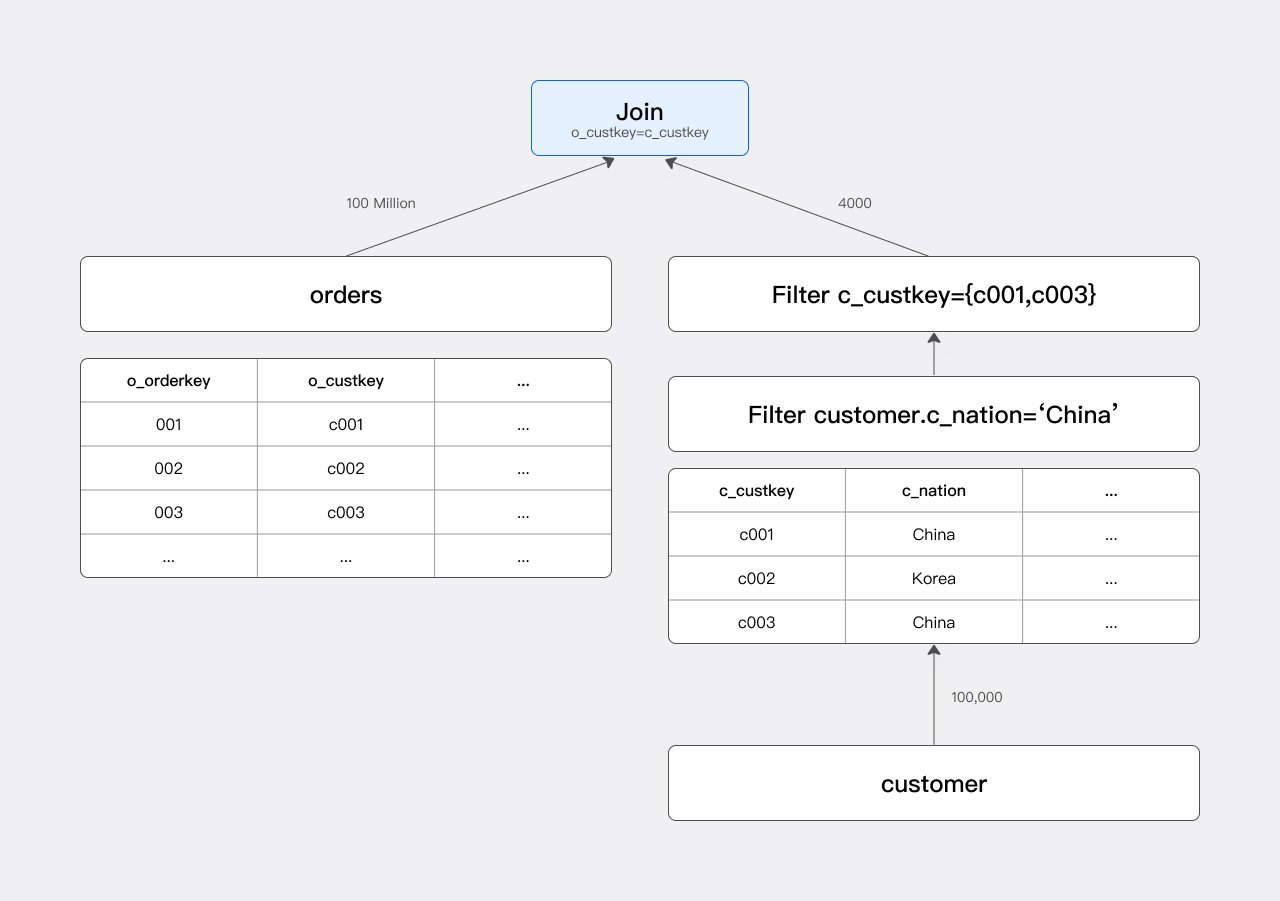
Without JRF: The Scan node scans the orders table, reading 100 million rows of data. The Join node then performs a Hash Probe on these 100 million rows to generate the Join result.
1. Optimization
The filter condition c_nation = 'china' filters out all non-Chinese customers, so only a portion (approximately 1/25) of the customer table is involved in the Join. Given the subsequent Join condition o_custkey = c_custkey, we need to focus on the c_custkey values selected in the filtered result. Let's denote the filtered c_custkey values as set A. In the following text, we use set A specifically to refer to the c_custkey set participating in the Join.
If set A is pushed down to the orders table as an IN condition, the Scan node for the orders table can filter the orders accordingly. This is similar to adding a filter condition o_custkey IN (c001, c003).
Based on this optimization concept, SQL can be optimized to:
select count(*)
from orders join customer on o_custkey = c_custkey
where c_nation = "china" and o_custkey in (c001, c003)
The optimized execution plan is illustrated below:

By adding a filter condition on the orders table, the actual number of orders participating in the Join is reduced from 100 million to 400,000, significantly improving query speed.
2. Implementation
While the optimization described above is significant, the optimizer does not know the actual c_custkey values selected (set A) and thus cannot statically generate a fixed in-predicate filter operator during the optimization phase.
In practical applications, we collect the right-side data at the Join node, generate set A at runtime, and push down set A to the Scan node of the orders table. We typically denote this JRF as: RF(c_custkey -> [o_custkey]).
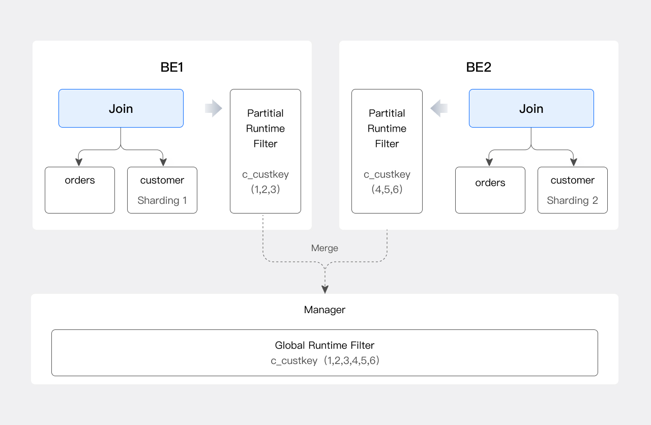
As Doris is a distributed database, JRF requires an additional merging step to cater to distributed scenarios. Assuming the Join in the example is a Shuffle Join, multiple instances of this Join handle individual shards of the orders and customer tables. Consequently, each Join instance only obtains a portion of set A.
In the current version of Doris, we select a node to serve as the Runtime Filter Manager. Each Join instance generates a Partial JRF based on the c_custkey values in its shard and sends it to the Manager. The Manager collects all Partial JRFs, merges them into a Global JRF, and then sends the Global JRF to all Scan instances of the orders table.
The process of generating the Global JRF is illustrated below:
Filter Types
There are various data structures that can be employed to implement JRF (Join Runtime Filter), each with varying efficiencies in generation, merging, transmission, and application, making them suitable for different scenarios.
1. In Filter
The simplest approach to implementing JRF is through the use of an In Filter. Taking the previous example, when using an In Filter, the execution engine generates a predicate o_custkey in (...list of elements in Set A...) on the left table. This In filter condition can then be applied to filter the orders table. When the number of elements in Set A is small, the In Filter is efficient.
However, using an In Filter becomes problematic when the number of elements in Set A is large:
-
Firstly, the cost of generating an In Filter is high, especially when JRF merging is required. Values collected from Join nodes corresponding to different data partitions may contain duplicates. For instance, if
c_custkeyis not the primary key of the table, values likec001andc003could appear multiple times, necessitating a time-consuming deduplication process. -
Secondly, when Set A contains many elements, the cost of transmitting data between the Join node and the Scan node of the orders table is significant.
-
Lastly, executing the In predicate at the Scan node of the orders table also takes time.
Considering these factors, we introduce the Bloom Filter.
2. Bloom Filter
For those unfamiliar with Bloom Filters, they can be thought of as a set of superimposed hash tables. Using a Bloom Filter (or hash table) for filtering leverages the following property:
-
A hash table T is generated based on Set A. If an element is not in hash table T, it can be definitively concluded that the element is not in Set A. However, the reverse is not true.
Therefore, if an
o_orderkeyis filtered out by the Bloom Filter, it can be concluded that there is no matchingc_custkeyon the right side of the Join. Nevertheless, due to hash collisions, someo_custkeys may pass through the Bloom Filter even if there is no matchingc_custkey.While a Bloom Filter cannot achieve precise filtering, it still provides a certain level of filtering effectiveness.
-
The number of buckets in the hash table determines the accuracy of filtering. The larger the number of buckets, the larger and more accurate the Filter becomes, but at the cost of increased computational overhead in generation, transmission, and usage.
Therefore, the size of the Bloom Filter must strike a balance between filtering effectiveness and usage costs. To this end, we have set a configurable range for the Bloom Filter's size, defined by
RUNTIME_BLOOM_FILTER_MIN_SIZEandRUNTIME_BLOOM_FILTER_MAX_SIZE.
3. Min/Max Filter
Apart from the Bloom Filter, the Min-Max Filter can also be used for approximate filtering. If the data column is ordered, the Min-Max Filter can achieve excellent filtering results. Additionally, the costs of generating, merging, and using a Min-Max Filter are significantly lower than those of an In Filter or Bloom Filter.
For non-equi Joins, both In Filters and Bloom Filters become ineffective, but the Min-Max Filter can still function. Suppose we modify the query from the previous example to:
select count(*)
from orders join customer on o_custkey > c_custkey
where c_name = "China"
In this case, we can select the maximum filtered c_custkey, denote it as n, and pass it to the Scan node of the orders table. The Scan node will then only output rows where o_custkey > n.
Viewing Join Runtime Filter
To see which JRFs (Join Runtime Filters) have been generated for a specific query, you can use the explain, explain shape plan, or explain physical plan commands.
Using the TPC-H Schema as an example, we will detail how to view JRFs using these three commands.
select count(*) from orders join customer on o_custkey=c_custkey;
1. Explain
In traditional Explain output, JRF information is typically displayed in Join and Scan nodes, as shown in the following example:
4: VHASH JOIN(258)
| join op: INNER JOIN(PARTITIONED)[]
|  equal join conjunct: (o_custkey[#10] = c_custkey[#0])
|  runtime filters: RF000[bloom] <- c_custkey[#0] (150000000/134217728/16777216)
|  cardinality=1,500,000,000
|  vec output tuple id: 3
|  output tuple id: 3
|  vIntermediate tuple ids: 2
|  hash output slot ids: 10
|  final projections: o_custkey[#17]
|  final project output tuple id: 3
|  distribute expr lists: o_custkey[#10]
|  distribute expr lists: c_custkey[#0]
|
|---1: VEXCHANGE
|      offset: 0
|      distribute expr lists: c_custkey[#0]
3: VEXCHANGE
|  offset: 0
|  distribute expr lists:

PLAN FRAGMENT 2
| PARTITION: HASH_PARTITIONED: o_orderkey[#8]
| HAS_COLO_PLAN_NODE: false
| STREAM DATA SINK
|   EXCHANGE ID: 03
|   HASH_PARTITIONED: o_custkey[#10]

2: VOlapScanNode(242)
|  TABLE: regression_test_nereids_tpch_shape_sf1000_p0.orders(orders)
|  PREAGGREGATION: ON
|  runtime filters: RF000[bloom] -> o_custkey[#10]
|  partitions=1/1 (orders)
|  tablets=96/96, tabletList=54990,54992,54994 ...
|  cardinality=0, avgRowSize=0.0, numNodes=1
|  pushAggOp=NONE
-
Join Side:
runtime filters: RF000[bloom] <- c_custkey[#0] (150000000/134217728/16777216)This indicates that a Bloom Filter with ID 000 has been generated, using
c_custkeyas input to create the JRF. The three numbers following are related to Bloom Filter size calculations and can be ignored for now. -
Scan Side:
runtime filters: RF000[bloom] -> o_custkey[#10]This indicates that JRF 000 will be applied to the Scan node of the orders table, filtering the
o_custkeyfield.
2. Explain Shape Plan
In the Explain Plan series, we'll use Shape Plan as an example to show how to view JRFs.
mysql> explain shape plan select count(*) from orders join customer on o_custkey=c_custkey where c_nationkey=5;
+--------------------------------------------------------------------------------------------------------------------------+
Explain String(Nereids Planner)                                                                                            |
+--------------------------------------------------------------------------------------------------------------------------+
PhysicalResultSink                                                                                                         |
--hashAgg[GLOBAL]                                                                                                          |
----PhysicalDistribute[DistributionSpecGather]                                                                             |
------hashAgg[LOCAL]                                                                                                       |
--------PhysicalProject                                                                                                    |
----------hashJoin[INNER_JOIN shuffle]                                                                                     |
------------hashCondition=((orders.o_custkey=customer.c_custkey)) otherCondition=() buildRFs:RF0 c_custkey->[o_custkey]    |
--------------PhysicalProject                                                                                              |
----------------Physical0lapScan[orders] apply RFs: RF0                                                                    |
--------------PhysicalProject                                                                                              |
----------------filter((customer.c_nationkey=5))                                                                           |
------------------Physical0lapScan[customer]                                                                               |
+--------------------------------------------------------------------------------------------------------------------------+
11 rows in set (0.02 sec)
As shown above:
-
Join Side:
build RFs: RF0 c_custkey -> [o_custkey]indicates that JRF 0 is generated usingc_custkeydata and applied too_custkey. -
Scan Side:
PhysicalOlapScan[orders] apply RFs: RF0indicates that orders table is filtered by JRF 0.
3. Profile
During actual execution, BE outputs JRF usage details to the Profile (requires set enable_profile=true). Using the same SQL query as an example, we can view JRF execution details in the Profile.
-
Join Side
HASH_JOIN_SINK_OPERATOR  (id=3  ,  nereids_id=367):(ExecTime:  703.905us)
      -  JoinType:  INNER_JOIN
      。。。
      -  BuildRows:  617
      。。。
      -  RuntimeFilterComputeTime:  70.741us
      -  RuntimeFilterInitTime:  10.882us
This is the Build side Profile for the Join. In this example, generating the JRF took 70.741us with 617 rows of input data. The JRF size and type are shown on the Scan side.
-
Scan Side
OLAP_SCAN_OPERATOR  (id=2.  nereids_id=351.  table  name  =  orders(orders)):(ExecTime:  13.32ms)
            -  RuntimeFilters:  :  RuntimeFilter:  (id  =  0,  type  =  bloomfilter,  need_local_merge:  false,  is_broadcast:  true,  build_bf_cardinality:  false,
            。。。
            -  RuntimeFilterInfo:
                -  filter  id  =  0  filtered:  714.761K  (714761)
                -  filter  id  =  0  input:  747.862K  (747862)
            。。。
            -  WaitForRuntimeFilter:  6.317ms
          RuntimeFilter:  (id  =  0,  type  =  bloomfilter):
                -  Info:  [IsPushDown  =  true,  RuntimeFilterState  =  READY,  HasRemoteTarget  =  false,  HasLocalTarget  =  true,  Ignored  =  false]
                -  RealRuntimeFilterType:  bloomfilter
                -  BloomFilterSize:  1024
Note:
-
Lines 5-6 show the input rows and the number of filtered rows. A higher number of filtered rows indicates better JRF effectiveness.
-
Line 10,
IsPushDown = true, indicates that JRF computation has been pushed down to the storage layer, which can help reduce IO through delayed materialization. -
Line 10,
RuntimeFilterState = READY, indicates whether the Scan node has applied the JRF. Since JRF uses a try-best mechanism, if JRF generation takes too long, the Scan node may start scanning data after a waiting period, potentially outputting unfiltered data. -
Line 12,
BloomFilterSize: 1024, shows the size of the Bloom Filter in bytes.
-
Tuning
For Join Runtime Filter tuning, in most cases, the function is adaptive, and users do not need to manually tune it. However, there are a few adjustments that can be made to optimize performance.
1. Enable or Disable JRF
The session variable runtime_filter_mode controls whether JRFs are generated.
-
To enable JRF:
set runtime_filter_mode = GLOBAL -
To disable JRF:
set runtime_filter_mode = OFF
2. Set JRF Type
The session variable runtime_filter_type controls the type of JRFs, including:
-
IN(1) -
BLOOM(2) -
MIN_MAX(4) -
IN_OR_BLOOM(8)
The IN_OR_BLOOM Filter allows BE to adaptively choose between generating an IN Filter or a BLOOM Filter based on the actual number of rows of data.
Multiple JRF types can be generated for a single Join condition by setting runtime_filter_type to the sum of the corresponding enumeration values.
For example:
-
To generate both a
BLOOMFilter and aMIN_MAXFilter for each Join condition:set runtime_filter_type = 6 -
In version 2.1, the default value of
runtime_filter_typeis 12, which generates both aMIN_MAXFilter and anIN_OR_BLOOMFilter.
The integers in parentheses represent the enumeration values for Runtime Filter Types.
3. Set Wait Time
As mentioned earlier, JRF uses a Try-best mechanism, where Scan nodes wait for JRFs before starting. Doris calculates the wait time based on runtime conditions. However, in some cases, the calculated wait time may not be sufficient, resulting in JRFs not being fully effective, and the Scan nodes may output more rows than expected. As discussed in the Profile section, if RuntimeFilterState = false in the Scan node's Profile, users can manually set a longer wait time.
The session variable runtime_filter_wait_time_ms controls the wait time for Scan nodes to wait for JRFs. The default value is 1000 milliseconds.
4. Pruning JRF
In some cases, JRFs may not provide filtering benefits. For example, if the orders and customer tables have a primary-foreign key relationship, but there are no filtering conditions on the customer table, the input to the JRF would be all custkeys, allowing all rows in the orders table to pass through the JRF. The optimizer prunes ineffective JRFs based on column statistics.
The session variable enable_runtime_filter_prune = true/false controls whether pruning is performed. The default value is true.
TopN Runtime Filter
Principles
In Doris, data is processed in a block-streaming manner. Therefore, when an SQL statement includes a topN operator, Doris does not compute all results but instead generates a dynamic filter to pre-filter the data early on.
Consider the following SQL statement as an example:
select o_orderkey from orders order by o_orderdate limit 5;
The execution plan for this SQL statement is illustrated below:
mysql> explain select o_orderkey from orders order by o_orderdate limit 5;
+-----------------------------------------------------+
| Explain String(Nereids Planner)                     |
+-----------------------------------------------------+
| PLAN FRAGMENT 0                                     |
|   OUTPUT EXPRS:                                     |
|     o_orderkey[#11]                                 |
|   PARTITION: UNPARTITIONED                          |
|                                                     |
|   HAS_COLO_PLAN_NODE: false                         |
|                                                     |
|   VRESULT SINK                                      |
|      MYSQL_PROTOCAL                                 |
|                                                     |
|   2:VMERGING-EXCHANGE                               |
|      offset: 0                                      |
|      limit: 5                                       |
|      final projections: o_orderkey[#9]              |
|      final project output tuple id: 2               |
|      distribute expr lists:                         |
|                                                     |
| PLAN FRAGMENT 1                                     |
|                                                     |
|   PARTITION: HASH_PARTITIONED: O_ORDERKEY[#0]       |
|                                                     |
|   HAS_COLO_PLAN_NODE: false                         |
|                                                     |
|   STREAM DATA SINK                                  |
|     EXCHANGE ID: 02                                 |
|     UNPARTITIONED                                   |
|                                                     |
|   1:VTOP-N(119)                                     |
|   |  order by: o_orderdate[#10] ASC                 |
|   |  TOPN OPT                                       |
|   |  offset: 0                                      |
|   |  limit: 5                                       |
|   |  distribute expr lists: O_ORDERKEY[#0]          |
|   |                                                 |
|   0:VOlapScanNode(113)                              |
|      TABLE: tpch.orders(orders), PREAGGREGATION: ON |
|      TOPN OPT:1                                     |
|      partitions=1/1 (orders)                        |
|      tablets=3/3, tabletList=135112,135114,135116   |
|      cardinality=150000, avgRowSize=0.0, numNodes=1 |
|      pushAggOp=NONE                                 |
+-----------------------------------------------------+
41 rows in set (0.06 sec)
Without a topn filter, the scan node would sequentially read each data block from the orders table and pass them to the TopN node. The TopN node maintains the current top 5 rows from the orders table through heap sorting.
Since a data block typically contains around 1024 rows, the TopN node can identify the 5th ranked row within the first data block after processing it.
Assuming this o_orderdate is 1995-01-01, the scan node can then use 1995-01-01 as a filter condition when outputting the second data block, eliminating the need to send rows with o_orderdate greater than 1995-01-01 to the TopN node for further processing.
This threshold is dynamically updated. For instance, if the TopN node discovers a smaller o_orderdate when processing the second filtered data block, it updates the threshold to the fifth-ranked o_orderdate among the first two data blocks.
Viewing TopN Runtime Filter
Using the Explain command, we can inspect the TopN Runtime Filter planned by the optimizer.
1:VTOP-N(119)
| order by: o_orderdate[#10] ASC
| TOPN OPT
| offset: 0
| limit: 5
| distribute expr lists: O_ORDERKEY[#0]
|

0:VLapScanNode[113]
    TABLE: regression_test_nereids_tpch_p0.(orders), PREAGGREGATION: ON
    TOPN OPT: 1
    partitions=1/1 (orders)
    tablets=3/3, tabletList=135112,135114,135116
    cardinality=150000, avgRowSize=0.0, numNodes=1
    pushAggOp: NONE
As shown in the example above:
-
The TopN node displays
TOPN OPT, indicating that this TopN node generates a TopN Runtime Filter. -
The Scan node indicates which TopN node generates the TopN Runtime Filter it uses. For instance, in the example, line 11 indicates that the Scan node for the
orderstable will use the Runtime Filter generated by TopN node 1, shown asTOPN OPT: 1in the plan.
As a distributed database, Doris considers the physical machines where TopN and Scan nodes actually run. Due to the high cost of cross-BE communication, BEs adaptively decide whether and to what extent to use TopN Runtime Filters. Currently, we have implemented BE-level TopN Runtime Filters, where TopN and Scan reside on the same BE. This is because updating TopN Runtime Filter thresholds only requires inter-thread communication, which is relatively inexpensive.
Tuning
The session variable topn_opt_limit_threshold controls whether to generate a TopN Runtime Filter.
The fewer rows specified in the SQL's limit clause, the stronger the filtering effect of the TopN Runtime Filter. Therefore, by default, Doris enables the generation of corresponding TopN Runtime Filters only when the limit number is less than 1024.
For example, setting set topn_opt_limit_threshold=10 would prevent the generation of a TopN Runtime Filter for the following query:
select o_orderkey from orders order by o_orderdate limit 20;