Join
What is JOIN
In relational databases, data is distributed across multiple tables, which are interconnected through specific relationships. SQL JOIN operations allow users to combine different tables into a more complete result set based on these relationships.
JOIN types supported by Doris
-
INNER JOIN: Comparing each row of the left table with all rows of the right table based on the JOIN condition, returning matching rows from both tables. For more details, refer to the syntax definition for JOIN queries in SELECT.
-
LEFT JOIN: Building on the result set of an INNER JOIN, if a row from the left table does not have a match in the right table, all rows from the left table are returned, with corresponding columns from the right table shown as NULL.
-
RIGHT JOIN: The opposite of LEFT JOIN; if a row from the right table does not have a match in the left table, all rows from the right table are returned, with corresponding columns from the left table shown as NULL.
-
FULL JOIN: Building on the result set of an INNER JOIN, returning all rows from both tables, filling in NULL where there are no matches.
-
CROSS JOIN: Having no JOIN condition, returning the Cartesian product of the two tables, where each row from the left table is combined with each row from the right table.
-
LEFT SEMI JOIN: Comparing each row of the left table with all rows of the right table based on the JOIN condition. If a match exists, the corresponding row from the left table is returned.
-
RIGHT SEMI JOIN: The opposite of LEFT SEMI JOIN; comparing each row of the right table with all rows of the left table, returning the corresponding row from the right table if a match exists.
-
LEFT ANTI JOIN: Comparing each row of the left table with all rows of the right table based on the JOIN condition. If there is no match, the corresponding row from the left table is returned.
-
RIGHT ANTI JOIN: The opposite of LEFT ANTI JOIN; comparing each row of the right table with all rows of the left table, returning rows from the right table that do not have matches.
-
NULL AWARE LEFT ANTI JOIN: Similar to LEFT ANTI JOIN but ignoring rows in the left table where the matching column is NULL.
Implementation of JOIN in Doris
Doris supports two implementation methods for JOIN: Hash Join and Nested Loop Join.
- Hash Join: A hash table is built on the right table based on the equality JOIN columns, and the data from the left table is streamed through this hash table for JOIN calculations. This method is limited to cases where equality JOIN conditions are applicable.
- Nested Loop Join: This method uses two nested loops, driven by the left table, to iterate through each row of the left table and compare it with every row of the right table based on the JOIN condition. It is suitable for all JOIN scenarios, including those that Hash Join cannot handle, such as queries involving GREATER THAN or LESS THAN comparisons, or cases requiring Cartesian products. However, compared to Hash Join, Nested Loop Join may have inferior performance.
Implementation of Hash Join in Doris
As a distributed MPP database, Apache Doris requires data shuffling during the Hash Join process to ensure the correctness of the JOIN results. Below are several data shuffling methods:
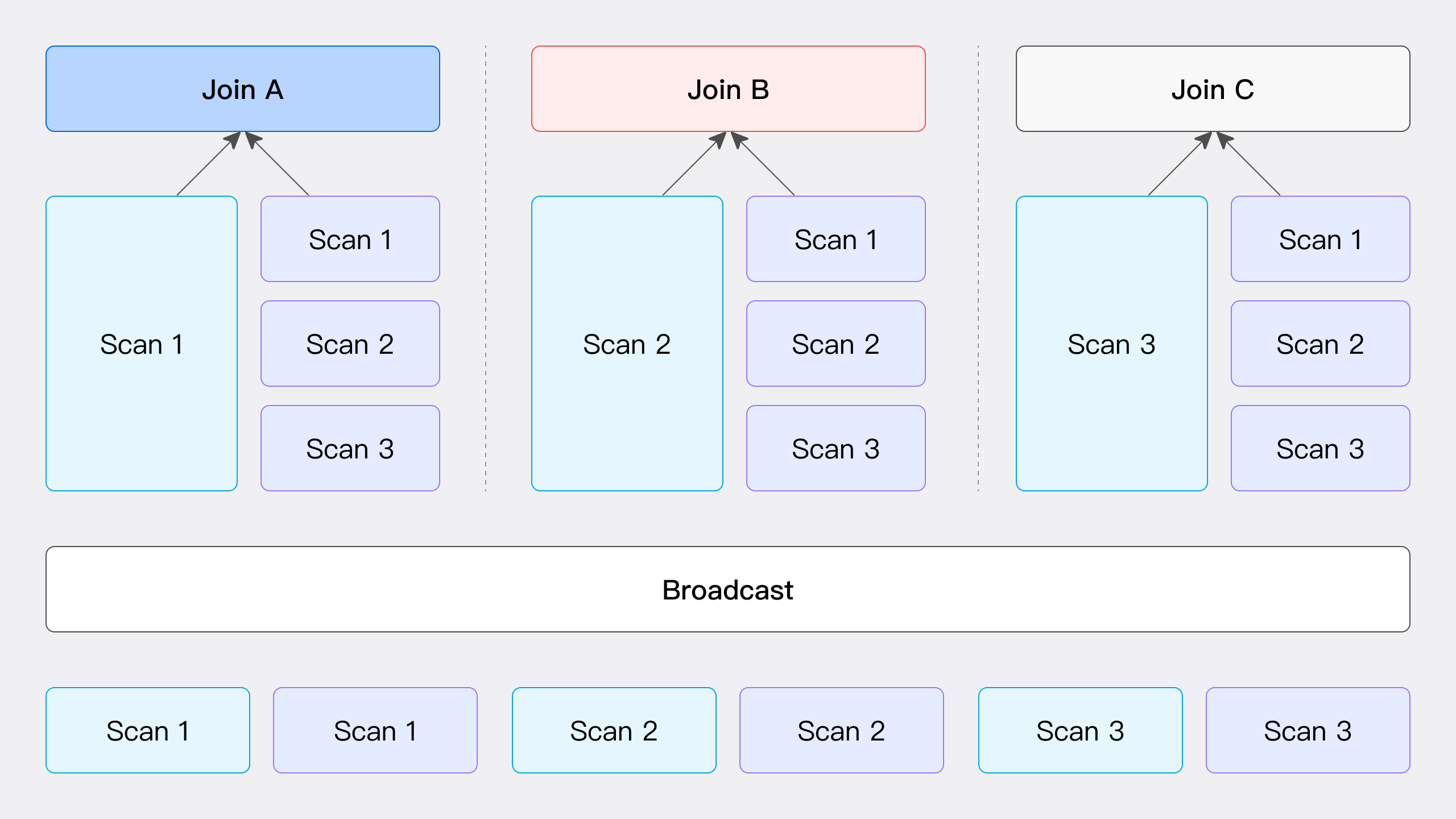
Broadcast Join As illustrated, the Broadcast Join process involves sending all data from the right table to all nodes participating in the JOIN computation, including the nodes scanning the left table data, while the left table data remains stationary. In this process, each node receives a complete copy of the right table's data (with a total volume of T(R)) to ensure that all nodes have the necessary data to perform the JOIN operation.
This method is suitable for various scenarios but is not applicable for RIGHT OUTER, RIGHT ANTI, and RIGHT SEMI types of Hash Join. Its network overhead is calculated as the number of JOIN nodes N multiplied by the volume of right table data T(R).
Partition Shuffle Join
This method computes hash values based on the JOIN conditions and performs bucketing. Specifically, the data from both the left and right tables is partitioned according to the hash values calculated from the JOIN conditions, and these partitioned data sets are then sent to the corresponding partition nodes (as illustrated).
The network overhead of this method mainly includes two parts: the cost of transferring the left table data T(S) and the cost of transferring the right table data T(R). This method only supports Hash Join operations because it relies on the JOIN conditions to perform data bucketing.

Bucket Shuffle Join
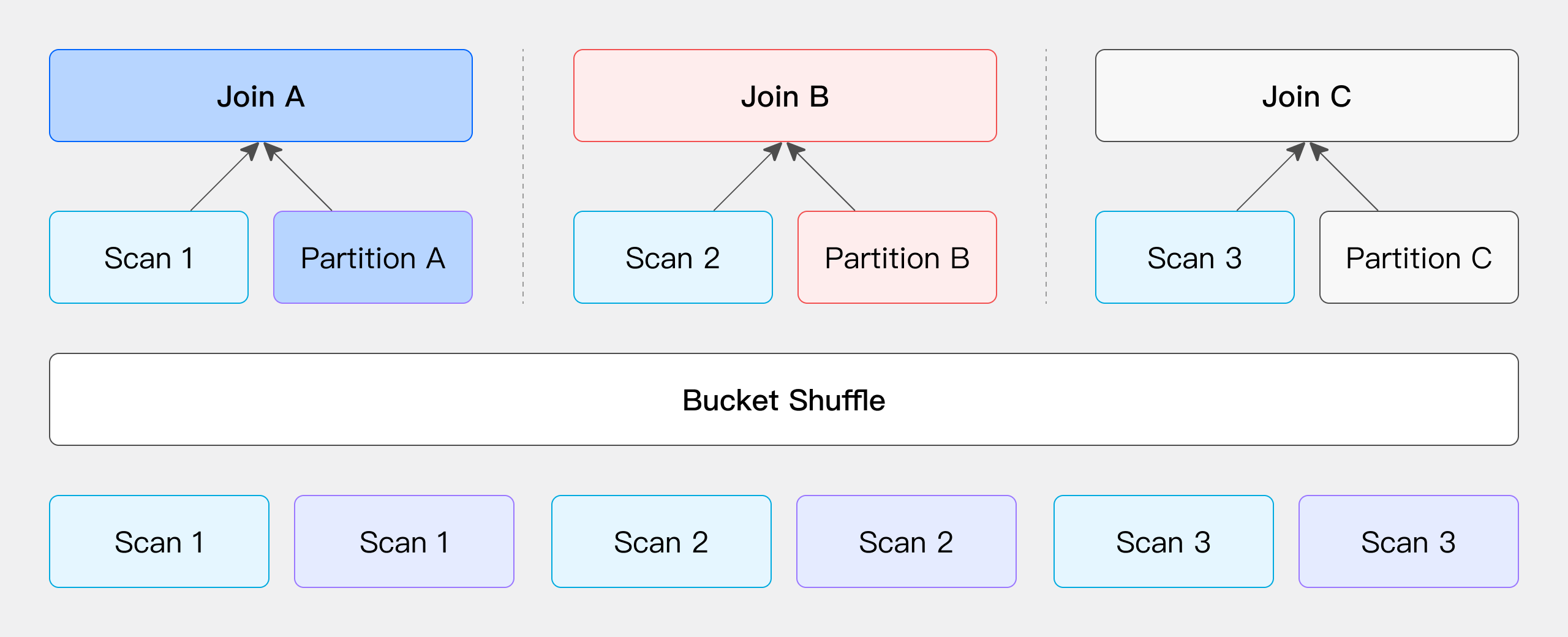
When the JOIN condition includes the bucketed column from the left table, the left table's data remains unchanged while the right table's data is distributed to the left table's nodes for the JOIN, reducing network overhead.
When one side of the table involved in the JOIN operation has its data already hash-distributed according to the JOIN condition column, users can choose to keep this side's data location unchanged while distributing the other side's data based on the same JOIN condition column and hash distribution. (The term "table" here refers not only to physically stored tables but also to the output results of any operators in SQL queries. Users can flexibly choose to keep either the left or right table's data location unchanged while only moving and distributing the other side's table.)
For example, in the case of physical tables of Doris, since the table data is stored in a bucketed manner through hash computation, users can directly leverage this feature to optimize the data shuffle process for the JOIN operation. Suppose you have two tables that need to be joined, and the JOIN column is the bucketed column from the left table. In this case, you do not need to move the left table's data; you only need to distribute the right table's data to the appropriate locations based on the left table's bucket information to complete the JOIN computation.
The primary network overhead for this process comes from the movement of the right table's data, denoted as T(R).
Colocate Join
Similar to Bucket Shuffle Join, if both tables involved in the Join are already distributed by Hash according to the Join condition columns, the Shuffle process can be skipped, and the Join calculation can be performed directly on the local data. This can be illustrated with physical tables:
When creating a table in Doris with the specification of DISTRIBUTED BY HASH, the system distributes data based on the Hash distribution key during data import. If the Hash distribution keys of both tables happen to match the Join condition columns, it can be said that the data in these two tables is already pre-distributed according to the Join requirements, eliminating the need for additional Shuffle operations. Therefore, during actual queries, the Join calculation can be executed directly on these two tables.
For scenarios where Join is executed after directly scanning data, certain conditions must be met during table creation; please refer to the subsequent restrictions regarding Colocate Join between the two physical tables.

Bucket Shuffle Join VS Colocate Join
As mentioned earlier, for both Bucket Shuffle Join and Colocate Join, the join operations can be executed as long as the distribution of the participating tables meets specific conditions (the term "tables" here refers to any output from SQL query operators).
Next, we will provide a more detailed explanation of the generalized Bucket Shuffle Join and Colocate Join using two tables, t1 and t2, along with relevant SQL examples. First, here are the table creation statements for both tables:
create table t1
(
    c1 bigint,
    c2 bigint
)
DISTRIBUTED BY HASH(c1) BUCKETS 3
PROPERTIES ("replication_num" = "1");

create table t2
(
    c1 bigint,
    c2 bigint
)
DISTRIBUTED BY HASH(c1) BUCKETS 3
PROPERTIES ("replication_num" = "1");
Example of Bucket Shuffle Join
In the following example, both tables t1 and t2 have been processed by the GROUP BY operator, resulting in new tables (at this point, the tx table is hash-distributed by c1, while the ty table is hash-distributed by c2). The subsequent JOIN condition is tx.c1 = ty.c2, which perfectly meets the conditions for a Bucket Shuffle Join.
explain select *
from
    (
        -- The t1 table is hash-distributed by c1, and after the GROUP BY operator, it still maintains the hash distribution by c1.
        select c1 as c1, sum(c2) as c2
        from t1
        group by c1
    ) tx
join
    (
        -- The t2 table is hash-distributed by c1, but after the GROUP BY operator, the data is redistributed to be hash-distributed by c2.
        select c2 as c2, sum(c1) as c1
        from t2
        group by c2
    ) ty
on tx.c1 = ty.c2;
From the following Explain execution plan, it can be observed that the left child node of the Hash Join node 7 is the aggregation node 6, while the right child node is the Exchange node 4. This indicates that the data from the left child node, after aggregation, remains in the same location, while the data from the right child node is distributed to the node where the left child node resides using the Bucket Shuffle method, in order to perform the subsequent Hash Join operation.
+------------------------------------------------------------+
| Explain String(Nereids Planner)                            |
+------------------------------------------------------------+
| PLAN FRAGMENT 0                                            |
|   OUTPUT EXPRS:                                            |
|     c1[#18]                                                |
|     c2[#19]                                                |
|     c2[#20]                                                |
|     c1[#21]                                                |
|   PARTITION: HASH_PARTITIONED: c1[#8]                      |
|                                                            |
|   HAS_COLO_PLAN_NODE: true                                 |
|                                                            |
|   VRESULT SINK                                             |
|      MYSQL_PROTOCAL                                        |
|                                                            |
|   7:VHASH JOIN(364)                                        |
|   |  join op: INNER JOIN(BUCKET_SHUFFLE)[]                 |
|   |  equal join conjunct: (c1[#12] = c2[#6])               |
|   |  cardinality=10                                        |
|   |  vec output tuple id: 8                                |
|   |  output tuple id: 8                                    |
|   |  vIntermediate tuple ids: 7                            |
|   |  hash output slot ids: 6 7 12 13                       |
|   |  final projections: c1[#14], c2[#15], c2[#16], c1[#17] |
|   |  final project output tuple id: 8                      |
|   |  distribute expr lists: c1[#12]                        |
|   |  distribute expr lists: c2[#6]                         |
|   |                                                        |
|   |----4:VEXCHANGE                                         |
|   |       offset: 0                                        |
|   |       distribute expr lists: c2[#6]                    |
|   |                                                        |
|   6:VAGGREGATE (update finalize)(342)                      |
|   |  output: sum(c2[#9])[#11]                              |
|   |  group by: c1[#8]                                      |
|   |  sortByGroupKey:false                                  |
|   |  cardinality=10                                        |
|   |  final projections: c1[#10], c2[#11]                   |
|   |  final project output tuple id: 6                      |
|   |  distribute expr lists: c1[#8]                         |
|   |                                                        |
|   5:VOlapScanNode(339)                                     |
|      TABLE: tt.t1(t1), PREAGGREGATION: ON                  |
|      partitions=1/1 (t1)                                   |
|      tablets=1/1, tabletList=491188                        |
|      cardinality=21, avgRowSize=0.0, numNodes=1            |
|      pushAggOp=NONE                                        |
|                                                            |
| PLAN FRAGMENT 1                                            |
|                                                            |
|   PARTITION: HASH_PARTITIONED: c2[#2]                      |
|                                                            |
|   HAS_COLO_PLAN_NODE: true                                 |
|                                                            |
|   STREAM DATA SINK                                         |
|     EXCHANGE ID: 04                                        |
|     BUCKET_SHFFULE_HASH_PARTITIONED: c2[#6]                |
|                                                            |
|   3:VAGGREGATE (merge finalize)(355)                       |
|   |  output: sum(partial_sum(c1)[#3])[#5]                  |
|   |  group by: c2[#2]                                      |
|   |  sortByGroupKey:false                                  |
|   |  cardinality=5                                         |
|   |  final projections: c2[#4], c1[#5]                     |
|   |  final project output tuple id: 3                      |
|   |  distribute expr lists: c2[#2]                         |
|   |                                                        |
|   2:VEXCHANGE                                              |
|      offset: 0                                             |
|      distribute expr lists:                                |
|                                                            |
| PLAN FRAGMENT 2                                            |
|                                                            |
|   PARTITION: HASH_PARTITIONED: c1[#0]                      |
|                                                            |
|   HAS_COLO_PLAN_NODE: false                                |
|                                                            |
|   STREAM DATA SINK                                         |
|     EXCHANGE ID: 02                                        |
|     HASH_PARTITIONED: c2[#2]                               |
|                                                            |
|   1:VAGGREGATE (update serialize)(349)                     |
|   |  STREAMING                                             |
|   |  output: partial_sum(c1[#0])[#3]                       |
|   |  group by: c2[#1]                                      |
|   |  sortByGroupKey:false                                  |
|   |  cardinality=5                                         |
|   |  distribute expr lists: c1[#0]                         |
|   |                                                        |
|   0:VOlapScanNode(346)                                     |
|      TABLE: tt.t2(t2), PREAGGREGATION: ON                  |
|      partitions=1/1 (t2)                                   |
|      tablets=1/1, tabletList=491198                        |
|      cardinality=10, avgRowSize=0.0, numNodes=1            |
|      pushAggOp=NONE                                        |
|                                                            |
|                                                            |
| Statistics                                                 |
|  planed with unknown column statistics                     |
+------------------------------------------------------------+
97 rows in set (0.01 sec)
Example of Colocate Join
In the following example, both tables t1 and t2 have been processed by the GROUP BY operator, resulting in new tables (at this point, both tx and ty are hash-distributed by c2). The subsequent JOIN condition is tx.c2 = ty.c2, which perfectly meets the conditions for a Colocate Join.
explain select *
from
    (
        -- The t1 table is initially hash-distributed by c1, but after the GROUP BY operator, the data distribution changes to be hash-distributed by c2.
        select c2 as c2, sum(c1) as c1
        from t1
        group by c2
    ) tx
join
    (
        -- The t2 table is initially hash-distributed by c1, but after the GROUP BY operator, the data distribution changes to be hash-distributed by c2.
        select c2 as c2, sum(c1) as c1
        from t2
        group by c2
    ) ty
on tx.c2 = ty.c2;
From the results of the following Explain execution plan, it can be seen that the left child node of Hash Join node 8 is aggregation node 7, and the right child node is aggregation node 3, with no Exchange node present. This indicates that the aggregated data from both the left and right child nodes remains in its original location, eliminating the need for data movement and allowing the subsequent Hash Join operation to be performed directly locally.
+------------------------------------------------------------+
| Explain String(Nereids Planner)                            |
+------------------------------------------------------------+
| PLAN FRAGMENT 0                                            |
|   OUTPUT EXPRS:                                            |
|     c2[#20]                                                |
|     c1[#21]                                                |
|     c2[#22]                                                |
|     c1[#23]                                                |
|   PARTITION: HASH_PARTITIONED: c2[#10]                     |
|                                                            |
|   HAS_COLO_PLAN_NODE: true                                 |
|                                                            |
|   VRESULT SINK                                             |
|      MYSQL_PROTOCAL                                        |
|                                                            |
|   8:VHASH JOIN(373)                                        |
|   |  join op: INNER JOIN(PARTITIONED)[]                    |
|   |  equal join conjunct: (c2[#14] = c2[#6])               |
|   |  cardinality=10                                        |
|   |  vec output tuple id: 9                                |
|   |  output tuple id: 9                                    |
|   |  vIntermediate tuple ids: 8                            |
|   |  hash output slot ids: 6 7 14 15                       |
|   |  final projections: c2[#16], c1[#17], c2[#18], c1[#19] |
|   |  final project output tuple id: 9                      |
|   |  distribute expr lists: c2[#14]                        |
|   |  distribute expr lists: c2[#6]                         |
|   |                                                        |
|   |----3:VAGGREGATE (merge finalize)(367)                  |
|   |    |  output: sum(partial_sum(c1)[#3])[#5]             |
|   |    |  group by: c2[#2]                                 |
|   |    |  sortByGroupKey:false                             |
|   |    |  cardinality=5                                    |
|   |    |  final projections: c2[#4], c1[#5]                |
|   |    |  final project output tuple id: 3                 |
|   |    |  distribute expr lists: c2[#2]                    |
|   |    |                                                   |
|   |    2:VEXCHANGE                                         |
|   |       offset: 0                                        |
|   |       distribute expr lists:                           |
|   |                                                        |
|   7:VAGGREGATE (merge finalize)(354)                       |
|   |  output: sum(partial_sum(c1)[#11])[#13]                |
|   |  group by: c2[#10]                                     |
|   |  sortByGroupKey:false                                  |
|   |  cardinality=10                                        |
|   |  final projections: c2[#12], c1[#13]                   |
|   |  final project output tuple id: 7                      |
|   |  distribute expr lists: c2[#10]                        |
|   |                                                        |
|   6:VEXCHANGE                                              |
|      offset: 0                                             |
|      distribute expr lists:                                |
|                                                            |
| PLAN FRAGMENT 1                                            |
|                                                            |
|   PARTITION: HASH_PARTITIONED: c1[#8]                      |
|                                                            |
|   HAS_COLO_PLAN_NODE: false                                |
|                                                            |
|   STREAM DATA SINK                                         |
|     EXCHANGE ID: 06                                        |
|     HASH_PARTITIONED: c2[#10]                              |
|                                                            |
|   5:VAGGREGATE (update serialize)(348)                     |
|   |  STREAMING                                             |
|   |  output: partial_sum(c1[#8])[#11]                      |
|   |  group by: c2[#9]                                      |
|   |  sortByGroupKey:false                                  |
|   |  cardinality=10                                        |
|   |  distribute expr lists: c1[#8]                         |
|   |                                                        |
|   4:VOlapScanNode(345)                                     |
|      TABLE: tt.t1(t1), PREAGGREGATION: ON                  |
|      partitions=1/1 (t1)                                   |
|      tablets=1/1, tabletList=491188                        |
|      cardinality=21, avgRowSize=0.0, numNodes=1            |
|      pushAggOp=NONE                                        |
|                                                            |
| PLAN FRAGMENT 2                                            |
|                                                            |
|   PARTITION: HASH_PARTITIONED: c1[#0]                      |
|                                                            |
|   HAS_COLO_PLAN_NODE: false                                |
|                                                            |
|   STREAM DATA SINK                                         |
|     EXCHANGE ID: 02                                        |
|     HASH_PARTITIONED: c2[#2]                               |
|                                                            |
|   1:VAGGREGATE (update serialize)(361)                     |
|   |  STREAMING                                             |
|   |  output: partial_sum(c1[#0])[#3]                       |
|   |  group by: c2[#1]                                      |
|   |  sortByGroupKey:false                                  |
|   |  cardinality=5                                         |
|   |  distribute expr lists: c1[#0]                         |
|   |                                                        |
|   0:VOlapScanNode(358)                                     |
|      TABLE: tt.t2(t2), PREAGGREGATION: ON                  |
|      partitions=1/1 (t2)                                   |
|      tablets=1/1, tabletList=491198                        |
|      cardinality=10, avgRowSize=0.0, numNodes=1            |
|      pushAggOp=NONE                                        |
|                                                            |
|                                                            |
| Statistics                                                 |
|  planed with unknown column statistics                     |
+------------------------------------------------------------+
105 rows in set (0.06 sec)
Comparison of four shuffle methods
| Shuffle Methods | Network Overhead | Physical Operator | Applicable Scenarios |
|---|---|---|---|
| Broadcast | N * T(R) | Hash Join /Nest Loop Join | General |
| Shuffle | T(S) + T(R) | Hash Join | General |
| Bucket Shuffle | T(R) | Hash Join | JOIN condition includes the left table's bucketed column, with the left table being single-partitioned. |
| Colocate | 0 | Hash Join | JOIN condition includes the left table's bucketed column, and both tables belong to the same Colocate Group. |
N: Number of instances participating in the Join calculation
T(Relation): Number of tuples in the relation
The flexibility of the four Shuffle methods decreases in order, and their requirements for data distribution become increasingly strict. In most cases, as the requirements for data distribution increase, the performance of Join calculations tends to improve gradually. It is important to note that if the number of buckets in a table is small, Bucket Shuffle or Colocate Join may experience a decrease in performance due to lower parallelism, potentially resulting in slower performance than Shuffle Join. This is because the Shuffle operation can more effectively balance data distribution, thereby providing higher parallelism in subsequent processing.
FAQ
Bucket Shuffle Join and Colocate Join have specific limitations regarding data distribution and JOIN conditions when applied. Below, we will elaborate on the specific restrictions for each of these JOIN methods.
Limitations of Bucket Shuffle Join
When directly scanning two physical tables for a Bucket Shuffle Join, the following conditions must be met:
-
Equality Join condition: Bucket Shuffle Join is only applicable for scenarios where the JOIN condition is based on equality, as it relies on hash calculations to determine data distribution.
-
Inclusion of bucketed columns in equality conditions: The equality JOIN condition must include the bucketed columns from both tables. When the left table's bucketed column is used as the equality JOIN condition, it is more likely to be planned as a Bucket Shuffle Join.
-
Data type consistency: Since the hash value computation results differ for different data types, the data types of the left table's bucketed column and the right table's equality JOIN column must match; otherwise, the corresponding planning cannot occur.
-
Table type restrictions: Bucket Shuffle Join is only applicable to native OLAP tables in Doris. For external tables such as ODBC, MySQL, and ES, Bucket Shuffle Join cannot be effective when they are used as the left table.
-
Single Partition Requirement: For partitioned tables, since the data distribution may differ across partitions, Bucket Shuffle Join is only guaranteed to be effective when the left table is a single partition. Therefore, when executing SQL, it is advisable to use
WHEREconditions to enable partition pruning strategies whenever possible.
Limitations of Colocate Join
When directly scanning two physical tables, Colocate Join has stricter limitations compared to Bucket Shuffle Join. In addition to meeting all the conditions for Bucket Shuffle Join, the following requirements must also be satisfied:
-
Consistency of bucket column types and counts: Not only must the types of the bucketed columns match, but the number of buckets must also be the same to ensure data distribution consistency.
-
Consistency of table replicas: The number of replicas for the tables must be consistent.
-
Explicit specification of Colocation Group: A Colocation Group must be explicitly specified; only tables within the same Colocation Group can participate in a Colocate Join.
-
Unstable state during replica repair or balancing: During operations such as replica repair or balancing, the Colocation Group may be in an unstable state. In this case, the Colocate Join will degrade to a regular Join operation.